DEM contour tutorial
Generate contour isobands from DEMs using contourrs.contours_arrow
and visualize them with GeoPandas + Matplotlib.
We start with a synthetic Gaussian-peak DEM, then apply the same workflow to a real Mt. Rainier elevation model.
from pathlib import Path

import geopandas as gpd
import matplotlib.pyplot as plt
import numpy as np
import rasterio
from contourrs import contours_arrow
Synthetic DEM
Sum of three Gaussian peaks to simulate a mountain range.
size = 256
y, x = np.mgrid[-3 : 3 : complex(size), -3 : 3 : complex(size)]
dem = (
    np.exp(-(x**2 + y**2))
    + 0.7 * np.exp(-((x - 1.5) ** 2 + (y - 1) ** 2) / 0.5)
    + 0.5 * np.exp(-((x + 1.5) ** 2 + (y + 1.5) ** 2) / 0.8)
).astype(np.float32)

print(f"DEM shape: {dem.shape}, range: [{dem.min():.3f}, {dem.max():.3f}]")
DEM shape: (256, 256), range: [0.000, 1.003]
Extract contour isobands
Define elevation thresholds and use contours_arrow to produce
filled contour polygons (isobands) as an Arrow table.
Convert to a GeoDataFrame for easy plotting.
thresholds = [0.1, 0.3, 0.5, 0.7, 0.9, 1.1]

table = contours_arrow(dem, thresholds=thresholds)
gdf = gpd.GeoDataFrame.from_arrow(table)

print(f"Isobands: {len(gdf)} polygons")
print(f"Threshold values: {sorted(gdf['value'].unique())}")
gdf.head()
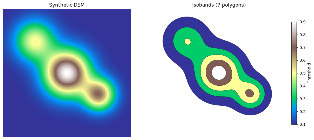
Isobands: 7 polygons
Threshold values: [np.float64(0.1), np.float64(0.3), np.float64(0.5), np.float64(0.7), np.float64(0.9)]
| geometry | value | |
|---|---|---|
| 0 | POLYGON ((15.519 65, 15.504 64, 15.511 63, 15.... | 0.1 |
| 1 | POLYGON ((36.505 65, 36.485 64, 36.501 63, 36.... | 0.3 |
| 2 | POLYGON ((59 65.488, 58.932 65, 58.948 64, 59 ... | 0.5 |
| 3 | POLYGON ((91.058 125, 91.038 124, 91.039 123, ... | 0.5 |
| 4 | POLYGON ((101.531 127, 101.516 126, 101.536 12... | 0.7 |
Synthetic raster and contour polygons
Side-by-side comparison of the continuous DEM and the filled contour bands.
h, w = dem.shape

fig, axes = plt.subplots(1, 2, figsize=(12, 5))

# Left: continuous DEM
axes[0].imshow(dem, cmap="terrain", interpolation="nearest", extent=(0, w, h, 0))
axes[0].set_title("Synthetic DEM")
axes[0].set_axis_off()
axes[0].set_xlim(0, w)
axes[0].set_ylim(h, 0)
axes[0].set_aspect("equal")

# Right: filled contour polygons
gdf.plot(
    ax=axes[1],
    column="value",
    cmap="terrain",
    edgecolor="black",
    linewidth=0.3,
    legend=True,
    legend_kwds={"label": "Threshold", "shrink": 0.8},
)
axes[1].set_title(f"Isobands ({len(gdf)} polygons)")
axes[1].set_axis_off()
axes[1].set_xlim(0, w)
axes[1].set_ylim(h, 0)
axes[1].set_aspect("equal")

plt.tight_layout()
plt.show()
Real DEM: Mt. Rainier
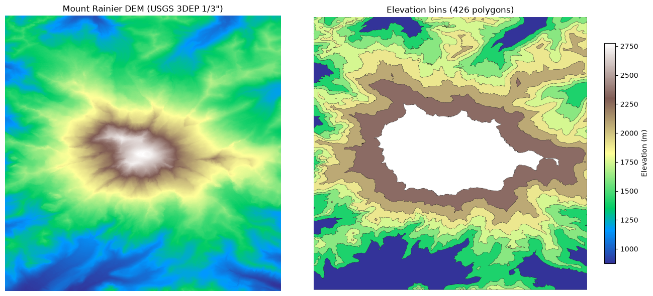
Apply the same contour workflow to a real 2048x2048 DEM of
Mt. Rainier (examples/data/mt_rainier_dem_2048.tif).
dem_path = Path("data/mt_rainier_dem_2048.tif")
if not dem_path.exists():
    dem_path = Path("examples/data/mt_rainier_dem_2048.tif")

with rasterio.open(dem_path) as src:
    real_dem = src.read(1)
    bounds = src.bounds
    nodata = src.nodata
    transform = src.transform

print(f"Shape: {real_dem.shape}, dtype: {real_dem.dtype}")
print(f"Elevation range: [{real_dem.min():.0f}, {real_dem.max():.0f}] m")
print(f"Bounds: {bounds}")
Shape: (2048, 2048), dtype: float32
Elevation range: [874, 4392] m
Bounds: BoundingBox(left=-121.8552777780595, bottom=46.758055555634236, right=-121.66564814822587, top=46.94768518546787)
Extract contours from Mt. Rainier
Use elevation thresholds spaced every 250 m.
# Mask out nodata
mask = np.ones(real_dem.shape, dtype=bool)
if nodata is not None:
    mask &= real_dem != nodata

valid = real_dem[mask]
vmin = float(valid.min())
vmax = float(valid.max())

# Quantile-based thresholds for visually balanced elevation bins
n_bins = 8
real_thresholds = [float(np.quantile(valid, q)) for q in np.linspace(0, 1, n_bins + 1)]
print(
    f"Thresholds ({len(real_thresholds)}):"
    f" {real_thresholds[0]:.0f} .. {real_thresholds[-1]:.0f} m"
)

real_table = contours_arrow(
    real_dem,
    thresholds=real_thresholds,
    nodata=nodata,
    transform=transform,
)
gdf_real = gpd.GeoDataFrame.from_arrow(real_table)

print(f"Elevation bins: {len(gdf_real)} polygons")
gdf_real.head()
Thresholds (9): 874 .. 4392 m


Elevation bins: 426 polygons
| geometry | value | |
|---|---|---|
| 0 | POLYGON ((-121.85528 46.9018, -121.85519 46.90... | 874.071167 |
| 1 | POLYGON ((-121.85528 46.87116, -121.85519 46.8... | 874.071167 |
| 2 | POLYGON ((-121.85528 46.84545, -121.85523 46.8... | 874.071167 |
| 3 | POLYGON ((-121.85528 46.8143, -121.85523 46.81... | 874.071167 |
| 4 | POLYGON ((-121.85528 46.79706, -121.85519 46.7... | 874.071167 |
Mt. Rainier raster and contour polygons
extent = (bounds.left, bounds.right, bounds.bottom, bounds.top)
h, w = real_dem.shape

fig, axes = plt.subplots(1, 2, figsize=(14, 6))

# Left: real DEM raster
axes[0].imshow(real_dem, cmap="terrain", interpolation="nearest", extent=extent)
axes[0].set_title('Mount Rainier DEM (USGS 3DEP 1/3")')
axes[0].set_axis_off()
axes[0].set_xlim(bounds.left, bounds.right)
axes[0].set_ylim(bounds.bottom, bounds.top)
axes[0].set_aspect("equal")

# Right: contour isobands
gdf_real.plot(
    ax=axes[1],
    column="value",
    cmap="terrain",
    edgecolor="black",
    linewidth=0.2,
    legend=True,
    legend_kwds={"label": "Elevation (m)", "shrink": 0.8},
)
axes[1].set_title(f"Elevation bins ({len(gdf_real)} polygons)")
axes[1].set_axis_off()
axes[1].set_xlim(bounds.left, bounds.right)
axes[1].set_ylim(bounds.bottom, bounds.top)
axes[1].set_aspect("equal")

plt.tight_layout()
plt.show()